Capital Markets and the Pricing of Risk

Lucas S. Macoris

Outline

• This lecture is mainly based the following textbooks:

  1. (Berk and DeMarzo 2023)
  2. (Brealey, Myers, and Allen 2020)

• Study review and practice: I strongly recommend using Prof. Henrique Castro (FGV-EAESP) materials. Below you can find the links to the corresponding exercises related to this lecture:

  1. Multiple Choice Exercises - click here
  2. Numeric Exercises - click here

\(\rightarrow\) For coding replications, whenever applicable, please follow this page or hover on the specific slides with coding chunks

Risk & Return: Insights from History

Risk & Return: Insights from History

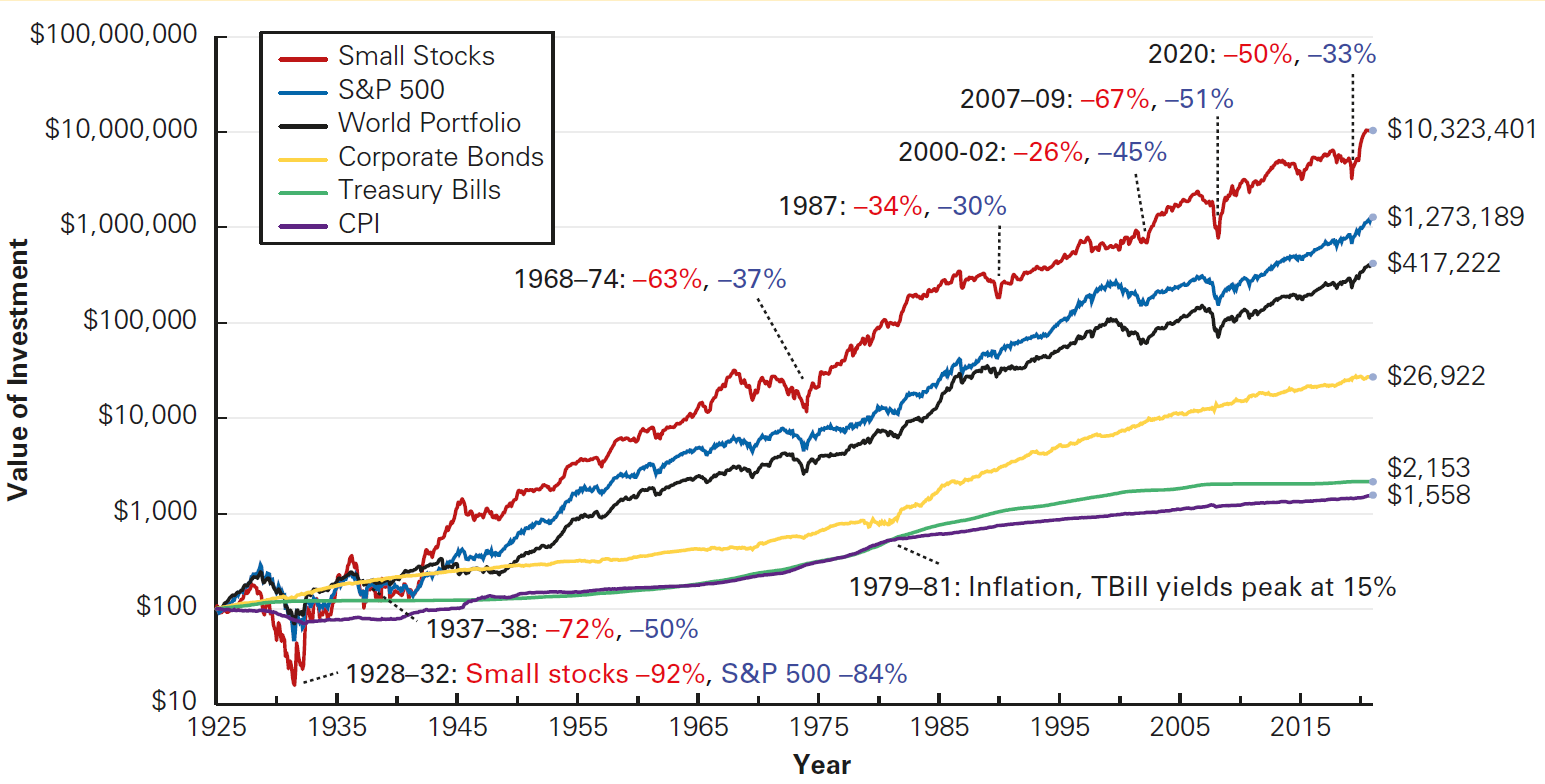
• There are a couple of observations based on historical data:

  1. Small stocks had the highest long-term return, while T-Bills had the lowest

  2. Small stocks had the largest fluctuations in price, while T-Bills had the lowest

  3. Higher risk requires a higher return

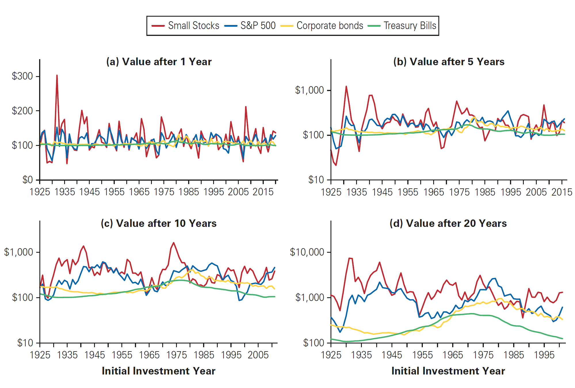
• More realistic investment horizons and different timeframes can greatly influence each investment’s risk and return over time

Risk & Return: Insights from History (continued)

Risk & Return: Insights from History (continued)

Measuring Risk and Return

Measures of Risk and Return

• If an investment is risky, it means that the return of its investment is not guaranteed:

1. Think about each possible return that a given investment can deliver. Each \(R\) has some likelihood (or probability) of occurring

2. This information is summarized with a probability distribution, which assigns a probability, \(P_{R}\) , that each possible return, \(R\), will occur

• For example, assume that a given stock currently trades for $100 per share. In one year, there is a 25% chance the share price will be 140, a 50% chance it will be 110, and a 25% chance it will be 80. The likelihood is then summarized as:

\[ \small P(R)= \begin{cases} 25\% \text{, for } R = 140, \\ 50\% \text{, for } R = 110, \\ 25\% \text{, for } R = 80, \\ \end{cases} \]

Measures of Risk and Return - Expected Returns

• Apart from the probability of occurrence, financial analysts are mostly interested in answering the following question: what is the expected return from a given investment?

Definition

Expected Return is the average of all possible returns, weighted by its return probability:

\[ E[R] = \sum_{R} P_R \times R \]

• In our simple example, we can compute expected returns as:

\[\small E[R_{BFI}] = 25\%\times(−0.20) + 50\%\times(0.10) + 25\%\times(0.40) = 10\%\]

Measures of Risk and Return - Standard Deviation

• Look at our previous example on BMA

  1. We know that \(E[R]=10\%\)
  2. Notwithstanding, looking at individual returns, there is significant variation from this average (or expected value)
  3. In other words, individual returns \(R\) can vary significantly from the expected value!

Definition

Stardard Deviation (Variance) of returns is the average deviation (average squared deviation) from the expected return:

\[Var(R) = E[(R-E[R])^2] = \sum_{R} P_R \times (R-E[R])^2 \]

\[SD(R) = \sqrt{Var(R)}\]

Measures of Risk and Return - Standard Deviation

• Using the previous example from BMA, we have that the variance of the returns can be computed as:

\[\text{Var}(R_{BMA}) = \sigma^2_{BMA}=0.25 × (−0.2 − 0.1)^2 + 0.5 × (0.1 − 0.1)^2 + 0.25 × (0.4 − 0.1)^2 = 0.045\]

• Therefore, the standard deviation of returns is simply:

\[SD(R_{BFI}) = \sigma_{BMA}= \sqrt{0.045} = 21.2\%\]

• In words: on average, we know that BMA return is 10%. Notwithstanding, the actual return can vary significantly - the average deviation from this expected return of 10% is \(\pm 21\%\).

Measures of Risk and Return - Caveats

• Expected Returns and the Variance (or the Standard Deviation) of returns are often used to characterize an asset in terms of risk and return. There are, notwithstanding, some caveats when we consider real cases of asset returns:

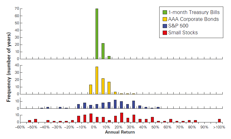
  1. Riskier assets, heavier tails: the likelihood of extreme negative or positive returns is bigger
  2. The standard Deviation of an assets changes over time
  3. Assets that are considered to be riskier tend to remain riskier than others

Important

Standard Deviation/Variance are correct measures of total risk only if the returns are normally distributed]{.blue}!

• Finally, keep in mind that the underlying assumption for using historical data is that past returns are good enough in predicting future returns, which may not hold!

Measures of Risk and Return - a global perspective

• As we saw, there seems to be a positive relationship between risk and return:

  1. Higher returns are generally associated with higher risk
  2. Lower returns, on the other hand, are less risky, and therefore more certain

• This assumption can also be externalized to different asset classes and/or markets:

  1. Stock market returns are higher and riskier than Treasury Bills
  2. Brazilian stock market returns are historically higher riskier than the U.S. stock market returns
  3. Brazilian Treasury Bill returns are historically higher and riskier than the U.S. Treasury Bill returns

Look at the difference in variationa cross asset classes!

Historical Returns

Historical Returns

• Our first example was a case where we knew the potential returns and their corresponding probabilities. With that, we were able to estimate the assets’ expected return

• In real-world applications, however, we do not know the potential returns and their probabilities. Because of that, the distribution of past returns can be helpful when we seek to estimate the distribution of returns investors may expect in the future

Definition

Therealized (or historical) return is the return that actually occurs over a particular time period. Suppose you invest in a stock on date \(t\) for price \(P_t\) . If the stock pays a dividend, \(Div_{t +1}\) , on date \(t + 1\), and you sell the stock at that time for price \(P_{t +1}\), then the realized return from your investment in the stock from \(t\rightarrow t + 1\) is:

\[R_{t+1} = \frac{\overbrace{Div_{t+1}}^{\text{Dividend yield}} + \overbrace{P_{t+1}}^{\text{Capital Gain}}}{P_t} - 1\]

A note on future value calculations

• Sometimes, we are interested in the compounded return over a longer period of time. Recall that the future value of an investment is given by:

\[ PV=\dfrac{FV}{(1+r)^n}\rightarrow FV = PV \times (1+r)^n \]

• Say that you observe a stock’s return for four periods: \(R_1,R_2,R_3\), and \(R_4\). How would you calculate the final price over the whole period (i.e, in \(t=4\))? The most straightforward way is to use the future value formula with \(PV\) equal to the price of a given stock in \(t=3\):

\[ FV= PV\times(1+r)^n \rightarrow P_4 = P_3\times(1+R_4)^1 \]

A note on future value calculations, continued

• By the same rationale, note that \(P_3\) is simply \(P_2\times(1+R_3)\). Iteratively, we have:

\[ \small P_4 = P_3\times(1+R_4)\\ \small P_4 = P_2\times(1+R_3)\times(1+R_4)\\ \small P_4 = P_1\times(1+R_2)\times\times(1+R_3)\times(1+R_4)\\ \small P_4 = \underbrace{P_0}_{\text{Initial Price}}\times\underbrace{(1+R_1)\times(1+R_2)\times(1+R_3)\times(1+R_4)}_{\text{Total Return for the Period}} \]

\(\rightarrow\) In words: the compounded return of a given asset over a period of time is just the product of all individual \((1+R_t)\)

Calculating realized annual returns

• Using the rationale presented before, if a stock pays dividends at the end of each quarter (with realized returns \(R_{Q1}\), \(R_{Q2}\), \(R_{Q3}\), and \(R_{Q4}\), then its annual realized return, \(R_{Annual}\), is computed as follows:

\[(1 + 𝑅_{Annual}) = (1+𝑅_{Q1})\times(1+𝑅_{Q2})\times(1+ 𝑅_{Q3})\times (1+𝑅_{Q4})\]

• Therefore, \(R_{Annual}\) (in percentage terms) is found subtracting by \(1\) from the previous formula

Important

You should know whether the return is calculated adjusted by dividends (they usually are, but always ask). For example, Yahoo! Finance provides Open, High, Low, Close, and Adjusted Close trading prices for each asset that is being tracked, where Adjusted Close is defined by the closing price adjusted for dividends and stock splits. If you use R, Python, or any API to pull this data, ensure to use the information adjusted by dividends and splits!

Example: Annual Historic Returns

• Compute the annual returns over \(2011\rightarrow 2012\) for this MSFT:

Date	Price ($)	Dividends ($)	Return
12/31/2011	58.69	-	-
1/31/2012	61.44	0.26	5.13%
4/30/2012	63.94	0.26	4.49%
7/31/2012	48.5	0.26	-23.74%
10/31/2012	54.88	0.29	13.75%
12/31/2012	53.31	0	-2.86%

\[𝑅_{2012}=(1.0513)\times(1.0449)\times(0.7626)\times(1.1375)\times(0.9714)−1=−7.43\%\]

Example: Annual Historic Returns, without dividends

Date	Price ($)	Dividends ($)	Return
12/31/2015	6.73	-	-
3/31/2016	5.72	-	-15.01%
6/30/2016	4.81	-	-15.91%
9/30/2016	5.20	-	8.11%
12/31/2016	2.29	-	-55.96%

\[ 𝑅_{2016}=(0.8499)\times(0.8409)\times(1.0811)\times(0.4404)−1=−65.9\%\]

• As the firm did not pay dividends in 2016, you can compute the annual return as:

\[\small \frac{2.29}{6.73}-1 = -65.9\%\]

Average Annual Return and Variance

Definition

The average annual return of an investment during some historical period is simply the average of the realized returns for each year.

\[\overline{R} = \frac{1}{T} (𝑅_1 + 𝑅_2 + ⋯ + 𝑅_𝑇) = \frac{1}{T} \sum_{t=1}^{T} R_t\]

Now, using the estimate for \(\overline{R}\), we can calculate the yearly variance and standard deviation as:

\[\small Var[R] = \frac{1}{T-1} \sum_{t=1}^{T} (R_t- \overline{R})^2 \]

\[\small SD(R) = \sqrt{Var(R)}\]

Important

Warning: because you are using a sample of historical returns (instead of the population) there is a T-1 in the variance formula. As \(T\rightarrow \infty\), then \(T-1 \rightarrow T\) and the sample variance approximates the population one.

Measures of Risk and Return - Practice

• Let’s use this rationale to calculate the expected returns from Petrobrás S.A (ticker: PETR3):

  1. Use the download link at the bottom of the page to download PETR3 monthly returns
  2. Plot the monthly returns over time. What do you see?
  3. Calculate the sample expected return by calculating the average monthly return over the period and add it to the chart
  4. Calculate the monthly volatility (or standard deviation of monthly returns)

Data Exercise

Because you don’t know the actual probabilities, you need to replace your expectation operator, \(E(\cdot)\), by a sample analogue - in our case, we calculate the expected returns as the sample average of past returns and the volatility as the sample standard deviation.

Data Exercise, continued

How acurate our average return estimate is?

• As you saw, we can use a security’s historical average return to estimate its actual expected return
• However, the historical average return is just an estimate of the expected return:
  1. If you change your sample (e.g, use different periods), the average return will change
  2. The historical average return may not be a good predictor of future return
• A way to assess such uncertainty is to estimate how much the average return is expected to change due to different samples

Definition

The standard error of the average return is given by:

\[SE(R) = \frac{SD(R)}{\sqrt{\text{Number of Observations}}}\]

Data Exercise - Standard Error

• From 2020 to 2024 (year-to-date), we have 62 months, and an sample standard deviation of returns of 11.72%

• Assume that the returns from PETR3 follow a normal distribution. You know from our statistics course that, for a normally-distributed random variable, a 95% confidence interval is corevered by \(\pm 1.96\) standard errors:

\[E[R] \pm 1.96\times SE = 1.12 \pm 1.96\times \dfrac{11.72}{\sqrt{62}}=[-1.8\%,+4.04\%]\]

• This means that, with 95% confidence interval, the expected return for PETR3 during this period ranges from -1.8% to 4.04%

Standard Error - another example

• From 1926 to 2017, the average return of the S&P 500 was 12.0%, with a standard deviation of 19.8%

\[E[R] \pm 1.96\times SE = 12\% \pm 1.96\times\frac{19.8\%}{\sqrt{92}}= 12\% \pm 4.05\%\]

• This means that, with 95% confidence interval, the expected return of the S&P 500 during this period ranges from 7.9% and 16.1%

• The longer the period, the more accurate you are. But even with 92 years of data, you are not very accurate to predict the expected return of the S&P500.

Compound Annual Growth Rate (CAGR)

1. Let’s get back to our example. Note that there are heavy tails, both negative and positive
2. Notwithstanding, a simple average return estimation gives the same weights to observations with small and big changes

• Because of that, some analysts prefer to use a geometric average instead of arithmetic average, also called Compound Annual Growth Rate or CAGR

Compound Annual Growth Rate (CAGR)

• CAGR is nothing more than the geometric average (instead of arithmetic):

\[\small CAGR = [(1+R_1)\times(1+R_2)\times ...\times (1+R_T)]^{\frac{1}{T}}-1\]

• Using our example, the geometric return of PETR3 is:

\[\small CAGR = \bigg[\prod_{i=1}^{62}(1+R_i)\bigg]^{\frac{1}{62}}-1\approx 0.38\%\]

• Remember the (arithmetic) average was 1.12%. Alternatively, we could have calculated the CAGR using Initial and Final Prices: \(\small CAGR = \bigg[\frac{\text{Final Price}}{\text{Initial Price}}\bigg]^\frac{1}{T}-1\)

Risk and Return

Trade-off between Risk and Return

• We saw that whenever average returns are higher, they’re generally riskier

• Relatedly, investors are assumed to be risk averse:

  1. To assume risk, they need extra return for that risk
  2. In other words, they demand excess returns relative to safer assets!

Definition

• Excess Return is difference between:
  1. The average return for an investment with risk; and
  2. The average return of a risk-free asset

1. The relationship is expected to be positve - higher excess returns should be accompained with higher volatility
2. In practice the association is not 100% linear as one might expect!

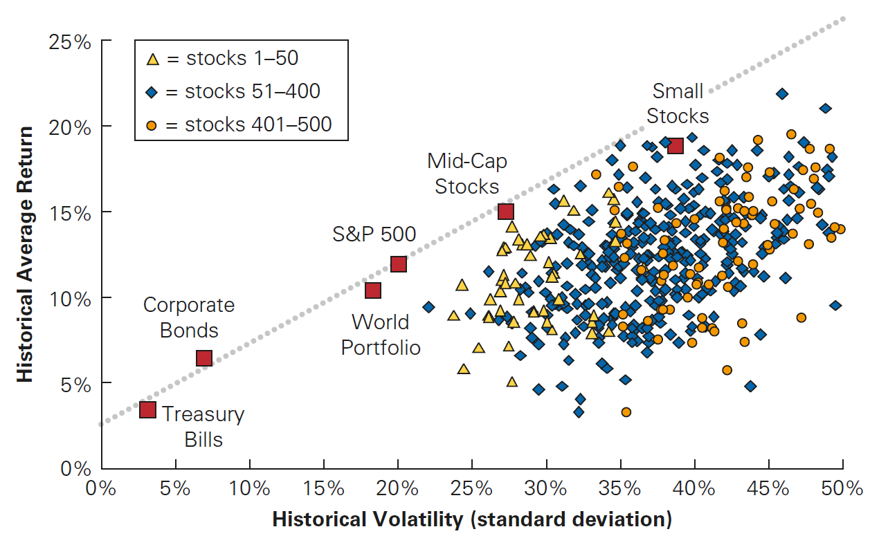
The tradeoff between risk and return in U.S. securities

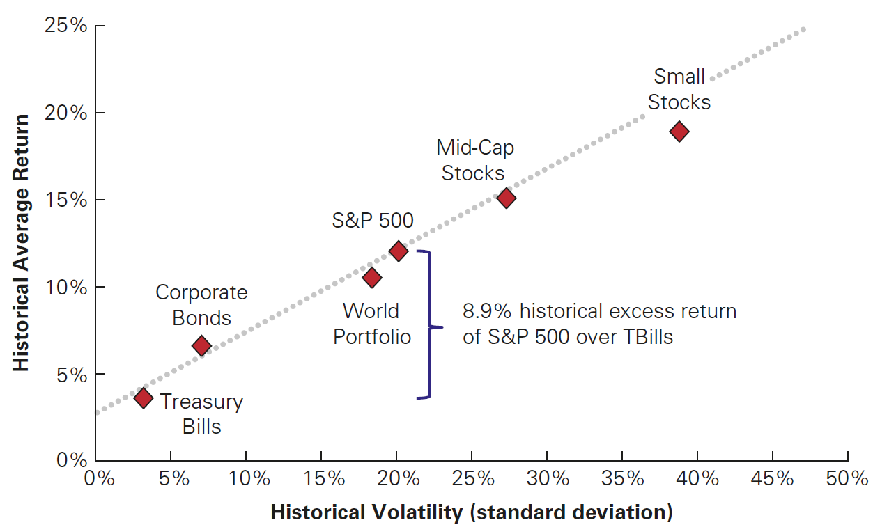
For individual stocks, there is no clear relationship!

Diversification

• As of now, we focused on a single asset case to analyze the risk and return

  1. In practice, investors hold a portfolio of assets
  2. How can we assess the portfolio average returns and its standard deviation?

• Why? Diversification! To see that, can think of risk in terms of two components:

  1. Firm-specific risk
     • Good or bad news about the company itself. For example, a firm might announce that it has been successful in gaining market share within its industry.
     • Also called firm-specific, idiosyncratic, unique, or diversifiable risk
  2. Market-wide risk
     • News about the economy as a whole, affects all assets
     • This type of risk is common to all firms
     • Also called systematic, undiversifiable, or market risk

Firm-specific versus systematic Risk

• When investors hold a portfolio of assets, the portfolio risk is lower than the weighted-average of the individual asset’s risks

• Why diversification works that way? The rationale behind the argument:

  1. When many stocks are combined in a large portfolio, the firm-specific risks for each stock will average out and be diversified
  2. The systematic risk, however, will affect all firms and will not be averaged out due to diversification!

• In practice, individual firms are affected by both market-wide risks and firm-specific risks

• When firms carry both types of risk, only the idiosyncratic risk will be diversified by forming a portfolio!

• This also explains why you haven’t found a clear risk \(\times\) return relationship between individual stocks, but when the firm-specific risk is eliminated (through portfolio formation), risk \(\times\) return comparison only consider the different exposure to systematic risks!

Firm-specific versus systematic Risk, continued

• To build on the previous point, consider two types of firms:

  • Type S firms are affected only by systematic risk
    1. There is a 50% chance the economy will be strong and they will earn a return of 40%
    2. There is a 50% change the economy will be weak and their return will be −20%
    3. Because all these firms face the same systematic risk, holding a large portfolio of type S firms will not diversify the risk
  • Type I firms are affected only by firm-specific risks
    1. Their returns are equally likely to be 35% or −25%, based on factors specific to each firm’s local market
    2. Because these risks are firm specific, if we hold a portfolio of many type I firms, risk is diversified!

Diversification - which risks are mitigated?

• Consider again Type I firms, which are affected only by firm-specific risk. Because each individual Type I firm is risky, should investors expect to earn a risk premium when investing in type I firms?

• The short answers is no, because the risk premium for diversifiable risk is zero, so investors are not compensated for holding firm-specific risk!

  1. The reason is that they can mitigate this part of risk through diversification
  2. Diversification eliminates this risk for free, implying that all investors should have a diversified portfolio. Otherwise, the investor is not rational

\(\rightarrow\) The key takeaway here is that the risk premium of a security is determined by solely by its systematic risk and does not depend on its diversifiable risk

Measures of Risk and Return - Practice

• Let’s use this rationale to understand how increasing the portfolio can reduce its volatility

  1. Use the download link at the bottom of the page to download a sample of daily returns for 10 selected stocks from Ibovespa
  2. Start from left to right and create a portfolio that consists of 100% of the first stock. Calculate the volatility of the returns. For \(n\geq2\), assign equal-weights to each stock
  3. Iterate until you have a portfolio comprised of \(10\) different stocks with 10% each
  4. Plot the annual volatility of each portfolio. How much were you able to reduce in terms of variance? How does this compare to an average volatility of the 10 stocks?

Data Exercise

Download the data using the following button and proceed with the practical exercise.

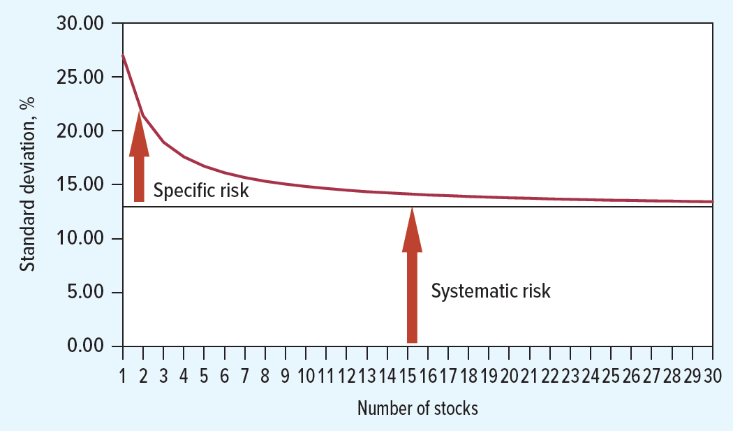
Limits to diversification

• How much volatility can we shrink through diversification? The volatility will therefore decline until only the systematic risk remains - e.g, exposure to macroeconomic events.

Diversification - wrapping-up

• All in all, in a world where diversification exists, the Standard Deviation is not a good measure for risk anymore:

  1. It is a measure a stock’s total risk, which includes diversifiable and non-diversifiable risks
  2. However, if you are diversified (and rationally, you should be), you are not incurring the total risk, only the systematic risk.

• Does that mean that standard deviation (or the variance) should never be used?

  1. No! Although the standard deviation of individual stocks contained in a portfolio is not a good measure of risk, the standard deviation of the returns of a portfolio itself is still a good measure for the portfolio’s risk
  2. Therefore, when comparing two portfolios, you are inherently comparing two “assets” that are already diversified, so the portfolio with the higher standard deviation is riskier!

Measuring Systematic Risk

Measuring Systematic Risk

• As we saw before, when it comes to diversification benefits, only the idiosyncratic risk can be diversified, whereas the systematic risk remains in place

• As a consequence, if you assume that diversification is possible, the standard deviation is not a good measure for risk anymore, as it mixes both types of risk: the one we can get rid out with diversification, and the one which we cannot get rid

• To measure the systematic risk of a stock, we need to quantity of the variability of its return is due to:

  1. Systematic Risk , or the portion that is not eliminated through diversification
  2. Idiosyncratic Risk, or the portion that can be eliminated through diversification

• Question: how can we decompose the risk into these components and extract the systematic part of a given stock’s risk?

Measuring Systematic Risk, continued

• To determine how sensitive a given stock \(S\) is to systematic risk, we can look at the average change in the return for each 1% change in the return of a portfolio that fluctuates solely due to systematic risk - which we’ll call \(R_M\) for now:

\[ \beta=\dfrac{\Delta \overline R_S}{\Delta \overline{R}_{M}} \]

• In other words, \(\beta\) measures the expected % change in the excess return of a security for a 1% change in the excess return of the market portfolio

Measuring Systematic Risk - estimating \(\beta\)

• Suppose the market portfolio tends to increase by +47% when the economy is strong and decline by -25% when the economy is weak. What is the beta of a Type S (i.e, with only systematic risk) firm whose return is +40% on average when the economy is strong and −20% when the economy is weak?

  1. If the Market increases by +47%, then Type S increases by +40% \(\rightarrow \beta = \frac{40}{47}=0.85\)
  2. If the Market decreases by -25%, then Type S decreases by -20% \(\rightarrow \beta = \frac{20}{25}=0.8\)
  3. If the Market changes from -25% to +47% = 72%, Type S changes from -20% to 40% \(\rightarrow \beta = \frac{60}{72}=0.833\)

• Important: it does not mean that the stock has three \(\beta\)’s. Rather, it just means that we have three estimates for the stock’s sensitivity to systematic risk (\(\beta\))

• Also, note that, using the the same setting as before, the \(\beta\) of a Type I firm that bears only idiosyncratic, firm-specific risk is zero: \(\beta=\frac{0}{72}=0\)

Market Risk Premium

• Let’s say that you decide to hold the exact market portfolio (e.g, buy an ETF that mimicks the S&P500, Dow Jones Index, or even the Ibovespa Index for a brazilian setting). By definition, because your portfolio is exactly the market portfolio, then \(\beta=1\)

• You know that, rationally, the higher the risk, the higher the return you need to earn in order to justify holding this portfolio (and not holding, for example, risk-free assets)

• The question that remains is…how much are you earning, in addition to a risk-free portfolio, for bearing systematic risk?

Definition

The Market (or Equity) Risk Premium (or MRP) is the reward investors expect to earn for holding a portfolio with a \(\beta\) of 1 - i.e, the market portfolio:

\[\text{MRP} = \underbrace{E[R_m]}_{\text{Return of the Market portfolio}} - \underbrace{R_{F}}_{\text{Return of a risk-free asset}}\]

Market Risk Premium, continued

• Note that MRP is an excess return: it is the return that investors receive net of what they would have earned if they invested in risk-free assets - investors are risk-averse and dislike risk
  1. Therefore, in order to invest in risky assets, investors demand an extra return
  2. Flipping the argument, a risky asset will have to pay an extra return for its additional risk in order to attract investors!

\[E[R_m] = R_{F} + MRP\]

\(\rightarrow\) Key Takeaway: the return of the market portfolio is simply the sum of the risk-free return and the premium for bearing systematic risk!

1. There is some heterogeneity in the market risk premium across countries
2. Furthermore, the Market Risk premium also changes over time due to macroeconomic conditions (for example, changes in SELIC)

Market Risk Premium - continued

• Estimating the historical Market excess returns is fairly straightforward:
  1. Define what the market portfolio is: it can be, for example, a representative index of a country’s stock exchange, such as the S&P500 (U.S) or Ibovespa (Brazil)
  2. Define what is the corresponding risk-free asset - in the U.S. case, we generally use the return on Treasury Bills and Treasury-Bonds - similar to Tesouro Direto in Brazil
• A word of caution: again, note that this is not the same as of the expected Market Risk Premium, which is forward-looking! In practice, we often compute the historical average return and using this number as the best estimate of the expected returns

Market Risk Premium - Sources

• You can find the Market Risk Premium estimation
  1. United States and other countries (A. Damodaran, NYU Stern): access here
  2. Brazil (CEQEF-FGV): access here

\(\beta\) and the Cost of Capital

Expected Returns for individual stocks

• Consider an investment with \(\beta = 1.5\)

  1. This investment has 50% more risk than the market portfolio
  2. Every 1% change in the market portfolio leads to a 1.5% percent change in the investment’s price

• Question: what is the expected return for investing in this specific stock? Based on these figures, we can compute the expected return for this investment, adjusted by the level or risk it provides:

\[E[R] = R_{rf} + \beta \times (E[R_m] - R_{rf})\]

• We will discuss more about this equation later when discussing the CAPM (or Capital Asset Pricing Model)

Example: \(\beta\) and the Cost of Capital

• Assume the economy has a 60% chance that the market return will be 15% next year and a 40% chance the market return will be 5% next year. Assume the risk-free rate is 6%. If a company’s beta is 1.18, what is its expected return next year?

  1. First, compute \(E[R_m]\):

\[ E[R_m] = 60\% \times 15\% + 40\% \times 5\% = 11\%\]

2. Second, compute \(E[R]\):

\[E[R] = 6\% + 1.18 \times (11\% - 6\%) = 11.9\%\]

\(\rightarrow\) Key Takeaway: because the stock riskier than the market portfolio, the risk-premium is also higher!

\(\beta\) for selected stocks (against Ibovespa)

Practice

Important

Practice using the following links:

1. Multiple-choice Questions
2. Numeric Questions

References

Berk, J., and P. DeMarzo. 2023. Corporate Finance, Global Edition. Global Edition / English Textbooks. Pearson. https://books.google.com.br/books?id=m78oEAAAQBAJ.

Brealey, R. A., S. C. Myers, and F. Allen. 2020. Principles of Corporate Finance. The Irwin/McGraw-Hill Series in Finance, Insurance, and Real Estate. McGraw-Hill Education. https://books.google.com.br/books?id=nsrHuwEACAAJ.